Solutions

(1) The easiest way to get the cumulative sum is using the built-in cumsum function, but we need to group the data by pickup_nb before applying it. Finally, we use filter to get on the top destination neighborhoods. The condition pct > 5 will give us only those neighborhoods that are a destination at least 5% of the time, and the condition (cumpct <= 50 | (cumpct > 50 & lag(cumpct) <= 50)) will stop us once the destinations together account for more than 50 percent of trips.

rxcs %>%
  select(pickup_nb, dropoff_nb, pct = pct_by_pickup_nb) %>%
  arrange(pickup_nb, desc(pct)) %>%
  group_by(pickup_nb) %>%
  mutate(cumpct = cumsum(pct)) %>%
  filter(pct > 5 & (cumpct <= 50 | (cumpct > 50 & lag(cumpct) <= 50))) %>%
  as.data.frame -> rxcs_tops

(2) We can use subset to extract the top drop-off neighborhoods for a given pick-up neighborhood. We use drop = TRUE the results into a vector. In the rxDataStep call, we can pass the two objects nb_name and nb_drop to the rowSelection argument by using transformObjects which is simply a named list. One quirk that we must be aware of here is that the objects (nb_name and nb_drop) must be renamed and the new names (nb and top_drop_for_nb respectively) go into rowSelection.

nb_name <- "West Village"
nb_drop <- subset(rxcs_tops, pickup_nb == nb_name, select = "dropoff_nb", drop = TRUE)

pickup_df <- rxDataStep(mht_xdf, 
                        rowSelection = pickup_nb == nb & dropoff_nb %in% top_drop_for_nb, 
                        varsToKeep = c("dropoff_nb", "tpep_pickup_datetime"),
                        transformObjects = list(nb = nb_name, top_drop_for_nb = nb_drop))

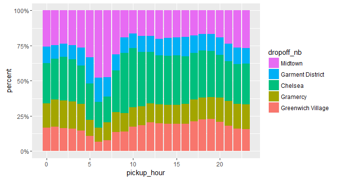
(3) We simply need to change position = "stack" to position = "fill". However, since the y-axis is mislabeled, we use scale_y_continuous(labels = percent_format()) and ylab("percent") to properly format and label the y-axis.

library(scales)
pickup_df %>%
  mutate(pickup_hour = hour(ymd_hms(tpep_pickup_datetime, tz = "UTC"))) %>%
  ggplot(aes(x = pickup_hour, fill = dropoff_nb)) +
  geom_bar(position = "fill", stat = "count") +
  scale_fill_discrete(guide = guide_legend(reverse = TRUE)) + 
  scale_y_continuous(labels = percent_format()) +
  ylab("percent")