Solutions

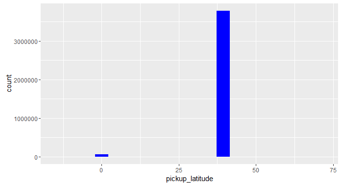
(1) As the plot shows, the latitude values also contain outliers and zeros.

ggplot(data = nyc_taxi) +
  geom_histogram(aes(x = pickup_latitude), fill = "blue", bins = 20)

(2) We can double-check the histogram for pickup_longitude by using cut and eyeballing the boundaries.

bucket_boundaries <- c(-Inf, -75, -73, -1, 1, Inf)
table(cut(nyc_taxi$pickup_longitude, bucket_boundaries))

(-Inf,-75]  (-75,-73]   (-73,-1]     (-1,1]   (1, Inf] 
        36    3785897         34      66395          0