Geographical features

The next set of features we extract from the data are geographical features, for which we load the following geospatial packages:

library(rgeos)
library(sp)
library(maptools)

It is common to store GIS data in R into shapefiles. A shapefile is essentially a data object that stores geospatial informaiton such as region names and boundaries where a region can be anything from a continent to city neighborhoods. The shapefile we use here was provided by Zillow.com and can be found here. It is a shapefile for the state of New York, and it contains neighborhood-level information for New York City.

nyc_shapefile <- readShapePoly('ZillowNeighborhoods-NY/ZillowNeighborhoods-NY.shp')

We can see what sort of information is available by peeking at nyc_shapefile@data:

head(nyc_shapefile@data, 10)

  STATE   COUNTY                        CITY            NAME REGIONID
0    NY   Monroe                   Rochester Ellwanger-Barry   343894
1    NY New York     New York City-Manhattan    West Village   270964
2    NY    Kings      New York City-Brooklyn     Bensonhurst   193285
3    NY     Erie                     Buffalo      South Park   270935
...

The data stores information about neighborhoods under the column NAME. Since we have longitude and latitude for pick-up and drop-off location, we can use the above data set to find the pick-up and drop-off neighborhoods for each cab ride. To keep the analysis simple, we limit the data to Manhattan only, where the great majority of cab rides take place.

nyc_shapefile <- subset(nyc_shapefile, COUNTY == 'New York') # limit the data to Manhattan only

Notice that even though nyc_shapefile is not a data.frame, subset still worked. This is because subset is a function that works on more than just one kind of input. Quite a few R functions are the same way, such as plot and predict.

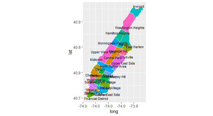
With a bit of work, we can plot a map of the whole area, showing the boundaries separating each neighborhood. We won't go into great detail on how the plots are generated, as it would derail us from the main topic.

library(ggplot2)
nyc_shapefile@data$id <- as.character(nyc_shapefile@data$NAME)
nyc_points <- fortify(gBuffer(nyc_shapefile, byid = TRUE, width = 0), region = "NAME") # fortify neighborhood boundaries

As part of the code to create the plot, we use dplyr to summarize the data and get median coordinates for each neighborhood, but since we revisit dplyr in greater depth in the next section, we skip the explanation for now.

library(dplyr)
nyc_df <- inner_join(nyc_points, nyc_shapefile@data, by = "id")
nyc_centroids <- summarize(group_by(nyc_df, id), long = median(long), lat = median(lat))

library(ggrepel)
library(ggplot2)
ggplot(nyc_df) + 
  aes(long, lat, fill = id) + 
  geom_polygon() +
  geom_path(color = "white") +
  coord_equal() +
  theme(legend.position = "none") +
  geom_text_repel(aes(label = id), data = nyc_centroids, size = 3)

We now go back to the data to find the neighborhood information based on the pick-up and drop-off coordinates. We store pick-up longitude and latitude in a separate data.frame, replacing NAs with zeroes (the function we're about to use doesn't work with NAs). We then use the coordinates function to point to the columns that correspond to the geographical coordinates. Finally, we use the over function to find the region (in this case the neighborhood) that the coordinates in the data fall into, and we append the neighborhood name as a new column to the nyc_taxi dataset.

data_coords <- data.frame(
  long = ifelse(is.na(nyc_taxi$pickup_longitude), 0, nyc_taxi$pickup_longitude), 
  lat = ifelse(is.na(nyc_taxi$pickup_latitude), 0, nyc_taxi$pickup_latitude)
)
coordinates(data_coords) <- c('long', 'lat') # we specify the columns that correspond to the coordinates
# we replace NAs with zeroes, becuase NAs won't work with the `over` function
nhoods <- over(data_coords, nyc_shapefile) # returns the neighborhoods based on coordinates
nyc_taxi$pickup_nhood <- nhoods$NAME # we attach the neighborhoods to the original data and call it `pickup_nhood`

We can use table to get a count of pick-up neighborhoods:

head(table(nyc_taxi$pickup_nhood, useNA = "ifany"))

      19th Ward Abbott McKinley        Albright           Allen       Annandale 
              0               0               0               0               0 
     Arbor Hill 
              0

We now repeat the above process, this using drop-off coordinates this time to get the drop-off neighborhood.

data_coords <- data.frame(
  long = ifelse(is.na(nyc_taxi$dropoff_longitude), 0, nyc_taxi$dropoff_longitude), 
  lat = ifelse(is.na(nyc_taxi$dropoff_latitude), 0, nyc_taxi$dropoff_latitude)
)
coordinates(data_coords) <- c('long', 'lat')
nhoods <- over(data_coords, nyc_shapefile)
nyc_taxi$dropoff_nhood <- nhoods$NAME

And since data_coords and nhoods are potentially large objects, we remove them from our session when they're no longer needed.

rm(data_coords, nhoods) # delete these objects, as they are no longer needed

Note how we had to repeat the same process in two different steps, once to get pick-up and once to get drop-off neighborhoods. Now if we need to change something about the above code, we have to change it in two different places. For example, if we want to reset the factor levels so that only Manhattan neighborhoods are showing, we need to remember to do it twice.

Another downside is we ended up with leftover objects data_coords and nhood. Since both objects have the same number of rows as the nyc_taxi dataset, they are relatively large objects, so we manually deleted them from the R session using rm after we finished using them. Carrying around too many by-product objects in the R session that are no longer needed can result in us clogging the memory, especially if the objects take up a lot of space. So we need to be careful and do some housecleaning every now and then so our session remains clean. Doing so is easier said than done.

There is however something we can do to avoid both of the above headaches: wrap the process into an R function.