Exercises

(1) The trim argument for the mean function is two-sided. Let's build a one- sided trimmed mean function, and one that uses counts instead of percentiles. Call it mean.minus.top.n. For example mean.minus.top.n(x, 5) will throw out the highest 5 values of x before computing the average. HINT: you can sort x using the sort function.

mean.minus.top.n(c(1, 5, 3, 99), 1) # should return 3

We just leared that the probs argument of quantile can be a vector. So instead of getting multiple quantiles separately, such as

c(quantile(nyc_taxi$trip_distance, probs = .9),
  quantile(nyc_taxi$trip_distance, probs = .6),
  quantile(nyc_taxi$trip_distance, probs = .3))

we can get them all at once by passing the percentiles we want as a single vector to probs:

quantile(nyc_taxi$trip_distance, probs = c(.3, .6, .9))

As it turns out, there's a considerable difference in efficiency between the first and second approach. We explore this in this exercise:

There are two important tools we can use when considering efficiency:

• profiling is a helpful tool if we need to understand what a function does under the hood (good for finding bottlenecks)
• benchmarking is the process of comparing multiple functions to see which is faster

Both of these tools can be slow when working with large datasets (especially the benchmarking tool), so instead we create a vector of random numbers and use that for testing (alternatively, we could use a sample of the data). We want the vector to be big enough that test result are stable (not due to chance), but small enough that they will run within a reasonable time frame.

random.vec <- rnorm(10^6) # a million random numbers generated from a standard normal distribution

Let's begin by profiling, for which we rely on the profr library:

library(profr)
my_test_function <- function(){
  quantile(random.vec, p = seq(0, 1, by = .01))
}
p <- profr(my_test_function())
plot(p)

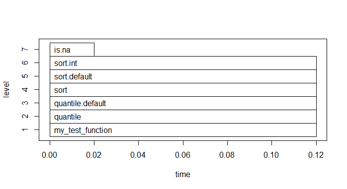
(2) Describe what the plot is telling us: what is the bottleneck in getting quantiles?

Now onto benchmarking, we compare two functions: first and scond. first finds the 30th, 60th, and 90th percentiles of the data in one function call, but scond uses three separate function calls, one for each percentile. From the profiling tool, we now know that every time we compute percentiles, we need to sort the data, and that sorting the data is the most time-consuming part of the calculation. The benchmarking tool should show that first is three times more efficient than scond, because first sorts the data once and finds all three percentiles, whereas scond sorts the data three different times and finds one of the percentiles every time.

first <- function(x) quantile(x, probs = c(.3, .6, .9)) # get all percentiles at the same time
scond <- function(x) {
  c(
    quantile(x, probs = .9),
    quantile(x, probs = .6),
    quantile(x, probs = .3))
}

library(microbenchmark) # makes benchmarking easy
print(microbenchmark(
  first(random.vec), # vectorized version
  scond(random.vec), # non-vectorized
  times = 10))

Unit: milliseconds
              expr   min    lq  mean median    uq   max neval
 first(random.vec)  62.7  68.9  78.2   75.8  89.8  97.4    10
 scond(random.vec) 119.8 130.3 139.3  140.7 146.9 157.6    10

(3) Describe what the results say? Do the runtimes bear out our intuition?